Copyright 2019 The TensorFlow Authors.
1 | #@title Licensed under the Apache License, Version 2.0 (the "License"); |
Transformer model for language understanding
View on TensorFlow.org | Run in Google Colab |  View source on GitHub |
This tutorial trains a Transformer model to translate Portuguese to English. This is an advanced example that assumes knowledge of text generation and attention.
The core idea behind the Transformer model is self-attention—the ability to attend to different positions of the input sequence to compute a representation of that sequence. Transformer creates stacks of self-attention layers and is explained below in the sections Scaled dot product attention and Multi-head attention.
A transformer model handles variable-sized input using stacks of self-attention layers instead of RNNs or CNNs. This general architecture has a number of advantages:
- It make no assumptions about the temporal/spatial relationships across the data. This is ideal for processing a set of objects (for example, StarCraft units).
- Layer outputs can be calculated in parallel, instead of a series like an RNN.
- Distant items can affect each other’s output without passing through many RNN-steps, or convolution layers (see Scene Memory Transformer for example).
- It can learn long-range dependencies. This is a challenge in many sequence tasks.
The downsides of this architecture are:
- For a time-series, the output for a time-step is calculated from the entire history instead of only the inputs and current hidden-state. This may be less efficient.
- If the input does have a temporal/spatial relationship, like text, some positional encoding must be added or the model will effectively see a bag of words.
After training the model in this notebook, you will be able to input a Portuguese sentence and return the English translation.

1 | from __future__ import absolute_import, division, print_function, unicode_literals |
/home/dongnanzhy/miniconda3/lib/python3.6/site-packages/h5py/__init__.py:36: FutureWarning: Conversion of the second argument of issubdtype from `float` to `np.floating` is deprecated. In future, it will be treated as `np.float64 == np.dtype(float).type`.
  from ._conv import register_converters as _register_converters
Setup input pipeline
Use TFDS to load the Portugese-English translation dataset from the TED Talks Open Translation Project.
This dataset contains approximately 50000 training examples, 1100 validation examples, and 2000 test examples.
1 | examples, metadata = tfds.load('ted_hrlr_translate/pt_to_en', with_info=True, |
[1mDownloading and preparing dataset ted_hrlr_translate (124.94 MiB) to /home/dongnanzhy/tensorflow_datasets/ted_hrlr_translate/pt_to_en/0.0.1...[0m
Failed to display Jupyter Widget of type HBox.
If you’re reading this message in the Jupyter Notebook or JupyterLab Notebook, it may mean
that the widgets JavaScript is still loading. If this message persists, it
likely means that the widgets JavaScript library is either not installed or
not enabled. See the Jupyter
Widgets Documentation for setup instructions.
If you’re reading this message in another frontend (for example, a static
rendering on GitHub or NBViewer),
it may mean that your frontend doesn’t currently support widgets.
WARNING: Logging before flag parsing goes to stderr.
W0525 16:13:27.155797 140479363516160 deprecation.py:323] From /home/dongnanzhy/miniconda3/lib/python3.6/site-packages/tensorflow_datasets/core/file_format_adapter.py:247: tf_record_iterator (from tensorflow.python.lib.io.tf_record) is deprecated and will be removed in a future version.
Instructions for updating:
Use eager execution and:
`tf.data.TFRecordDataset(path)`
Failed to display Jupyter Widget of type HBox.
If you’re reading this message in the Jupyter Notebook or JupyterLab Notebook, it may mean
that the widgets JavaScript is still loading. If this message persists, it
likely means that the widgets JavaScript library is either not installed or
not enabled. See the Jupyter
Widgets Documentation for setup instructions.
If you’re reading this message in another frontend (for example, a static
rendering on GitHub or NBViewer),
it may mean that your frontend doesn’t currently support widgets.
[1mDataset ted_hrlr_translate downloaded and prepared to /home/dongnanzhy/tensorflow_datasets/ted_hrlr_translate/pt_to_en/0.0.1. Subsequent calls will reuse this data.[0m
Create a custom subwords tokenizer from the training dataset.
1 | for pt, en in train_examples: |
tf.Tensor(b'agora aqui temos imagens sendo extra\xc3\xaddas em tempo real diretamente do feed ,', shape=(), dtype=string)
tf.Tensor(b'now here are live images being pulled straight from the feed .', shape=(), dtype=string)
b'now here are live images being pulled straight from the feed .'
1 | tokenizer_en = tfds.features.text.SubwordTextEncoder.build_from_corpus( |
1 | sample_string = 'Transformer is awesome.' |
Tokenized string is [7915, 1248, 7946, 7194, 13, 2799, 7877]
The original string: Transformer is awesome.
The tokenizer encodes the string by breaking it into subwords if the word is not in its dictionary.
Tensforflow Tokenizer自动把不在vocab里面的词按char level分开了,确保所有tokenize后的词都在vocab里
1 | for ts in tokenized_string: |
7915 ----> T
1248 ----> ran
7946 ----> s
7194 ----> former
13 ----> is
2799 ----> awesome
7877 ----> .
1 | BUFFER_SIZE = 20000 |
Add a start and end token to the input and target.
1 | def encode(lang1, lang2): |
Note: To keep this example small and relatively fast, drop examples with a length of over 40 tokens.
1 | MAX_LENGTH = 40 |
Operations inside .map() run in graph mode and receive a graph tensor that do not have a numpy attribute. The tokenizer expects a string or Unicode symbol to encode it into integers. Hence, you need to run the encoding inside a tf.py_function, which receives an eager tensor having a numpy attribute that contains the string value.
1 | def tf_encode(pt, en): |
1 | # Train set |
1 | de_batch, en_batch = next(iter(val_dataset)) |
(<tf.Tensor: id=311424, shape=(64, 40), dtype=int64, numpy=
 array([[8214, 1259,    5, ...,    0,    0,    0],
        [8214,  299,   13, ...,    0,    0,    0],
        [8214,   59,    8, ...,    0,    0,    0],
        ...,
        [8214,   95,    3, ...,    0,    0,    0],
        [8214, 5157,    1, ...,    0,    0,    0],
        [8214, 4479, 7990, ...,    0,    0,    0]])>,
 <tf.Tensor: id=311425, shape=(64, 40), dtype=int64, numpy=
 array([[8087,   18,   12, ...,    0,    0,    0],
        [8087,  634,   30, ...,    0,    0,    0],
        [8087,   16,   13, ...,    0,    0,    0],
        ...,
        [8087,   12,   20, ...,    0,    0,    0],
        [8087,   17, 4981, ...,    0,    0,    0],
        [8087,   12, 5453, ...,    0,    0,    0]])>)
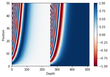
Positional encoding
Since this model doesn’t contain any recurrence or convolution, positional encoding is added to give the model some information about the relative position of the words in the sentence.
The positional encoding vector is added to the embedding vector. Embeddings represent a token in a d-dimensional space where tokens with similar meaning will be closer to each other. But the embeddings do not encode the relative position of words in a sentence. So after adding the positional encoding, words will be closer to each other based on the similarity of their meaning and their position in the sentence, in the d-dimensional space.
See the notebook on positional encoding to learn more about it. The formula for calculating the positional encoding is as follows:
$$\Large{PE_{(pos, 2i)} = sin(pos / 10000^{2i / d_{model}})} $$
$$\Large{PE_{(pos, 2i+1)} = cos(pos / 10000^{2i / d_{model}})} $$
1 | def get_angles(pos, i, d_model): |
1 | def positional_encoding(position, d_model): |
1 | pos_encoding = positional_encoding(50, 512) |
(1, 50, 512)
Masking
Mask all the pad tokens in the batch of sequence. It ensures that the model does not treat padding as the input. The mask indicates where pad value 0 is present: it outputs a 1 at those locations, and a 0 otherwise. (1代表被mask掉,0代表通过)
1 | def create_padding_mask(seq): |
1 | x = tf.constant([[7, 6, 0, 0, 1], [1, 2, 3, 0, 0], [0, 0, 0, 4, 5]]) |
<tf.Tensor: id=311442, shape=(3, 1, 1, 5), dtype=float32, numpy=
array([[[[0., 0., 1., 1., 0.]]],


       [[[0., 0., 0., 1., 1.]]],


       [[[1., 1., 1., 0., 0.]]]], dtype=float32)>
The look-ahead mask is used to mask the future tokens in a sequence. In other words, the mask indicates which entries should not be used.
This means that to predict the third word, only the first and second word will be used. Similarly to predict the fourth word, only the first, second and the third word will be used and so on.
look-ahead mask 确保sequence只能看到之前出现的word (1代表被mask掉,0代表通过)
1 | def create_look_ahead_mask(size): |
1 | x = tf.random.uniform((1, 3)) |
<tf.Tensor: id=311458, shape=(3, 3), dtype=float32, numpy=
array([[0., 1., 1.],
       [0., 0., 1.],
       [0., 0., 0.]], dtype=float32)>
Preprocessing finished
Scaled dot product attention
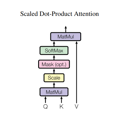
The attention function used by the transformer takes three inputs: Q (query), K (key), V (value). The equation used to calculate the attention weights is:
$$\Large{Attention(Q, K, V) = softmax_k(\frac{QK^T}{\sqrt{d_k}}) V} $$
d_k 代表K的dimension,这么做可以保证Q和K相乘后依然保留var=1. The dot-product attention is scaled by a factor of square root of the depth. This is done because for large values of depth, the dot product grows large in magnitude pushing the softmax function where it has small gradients resulting in a very hard softmax.
For example, consider that Q and K have a mean of 0 and variance of 1. Their matrix multiplication will have a mean of 0 and variance of dk. Hence, square root of dk is used for scaling (and not any other number) because the matmul of Q and K should have a mean of 0 and variance of 1, so that we get a gentler softmax.
mask乘以无穷小,0没有影响,表示通过。1变成无穷小,计算softmax后变成0,表示不通过. The mask is multiplied with -1e9 (close to negative infinity). This is done because the mask is summed with the scaled matrix multiplication of Q and K and is applied immediately before a softmax. The goal is to zero out these cells, and large negative inputs to softmax are near zero in the output.
1 | def scaled_dot_product_attention(q, k, v, mask): |
As the softmax normalization is done on K, its values decide the amount of importance given to Q.
The output represents the multiplication of the attention weights and the V (value) vector. This ensures that the words we want to focus on are kept as is and the irrelevant words are flushed out.
1 | def print_out(q, k, v): |
1 | np.set_printoptions(suppress=True) |
Attention weights are:
tf.Tensor([[0. 1. 0. 0.]], shape=(1, 4), dtype=float32)
Output is:
tf.Tensor([[10.  0.]], shape=(1, 2), dtype=float32)
1 | # This query aligns with a repeated key (third and fourth), |
Attention weights are:
tf.Tensor([[0.  0.  0.5 0.5]], shape=(1, 4), dtype=float32)
Output is:
tf.Tensor([[550.    5.5]], shape=(1, 2), dtype=float32)
1 | # This query aligns equally with the first and second key, |
Attention weights are:
tf.Tensor([[0.5 0.5 0.  0. ]], shape=(1, 4), dtype=float32)
Output is:
tf.Tensor([[5.5 0. ]], shape=(1, 2), dtype=float32)
Pass all the queries together.
1 | temp_q = tf.constant([[0, 10, 0], [0, 0, 10], [10, 10, 0]], dtype=tf.float32) # (3, 3) |
Attention weights are:
tf.Tensor(
[[0.  1.  0.  0. ]
 [0.  0.  0.5 0.5]
 [0.5 0.5 0.  0. ]], shape=(3, 4), dtype=float32)
Output is:
tf.Tensor(
[[ 10.    0. ]
 [550.    5.5]
 [  5.5   0. ]], shape=(3, 2), dtype=float32)
Multi-head attention
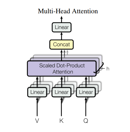
Multi-head attention consists of four parts:
- Linear layers and split into heads. (先把Q,K,V分成几个Heads)
- Scaled dot-product attention. (每个Head计算scaled dot-product attention)
- Concatenation of heads. (concat每个Head attn结果)
- Final linear layer. (再过一层FC[dimension 不变])
Each multi-head attention block gets three inputs; Q (query), K (key), V (value). These are put through linear (Dense) layers and split up into multiple heads.
The scaled_dot_product_attention defined above is applied to each head (broadcasted for efficiency). An appropriate mask must be used in the attention step. The attention output for each head is then concatenated (using tf.transpose, and tf.reshape) and put through a final Dense layer.
Instead of one single attention head, Q, K, and V are split into multiple heads because it allows the model to jointly attend to information at different positions from different representational spaces. After the split each head has a reduced dimensionality, so the total computation cost is the same as a single head attention with full dimensionality.
1 | class MultiHeadAttention(tf.keras.layers.Layer): |
Create a MultiHeadAttention layer to try out. At each location in the sequence, y, the MultiHeadAttention runs all 8 attention heads across all other locations in the sequence, returning a new vector of the same length at each location.
1 | temp_mha = MultiHeadAttention(d_model=512, num_heads=8) |
(TensorShape([1, 60, 512]), TensorShape([1, 8, 60, 60]))
Point wise feed forward network
Point wise feed forward network consists of two fully-connected layers with a ReLU activation in between.
1 | def point_wise_feed_forward_network(d_model, dff): |
1 | sample_ffn = point_wise_feed_forward_network(512, 2048) |
TensorShape([64, 50, 512])
Attention and Multi-Head module finished
Encoder and decoder
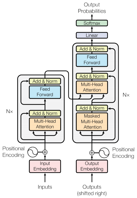
The transformer model follows the same general pattern as a standard sequence to sequence with attention model.
- The input sentence is passed through
Nencoder layers that generates an output for each word/token in the sequence. - The decoder attends on the encoder’s output and its own input (self-attention) to predict the next word.
Encoder layer
Each encoder layer consists of sublayers:
- Multi-head attention (with padding mask)
- Point wise feed forward networks.
Each of these sublayers has a residual connection around it followed by a layer normalization. Residual connections help in avoiding the vanishing gradient problem in deep networks.
The output of each sublayer is LayerNorm(x + Sublayer(x)). The normalization is done on the d_model (last) axis. There are N encoder layers in the transformer.
1 | class EncoderLayer(tf.keras.layers.Layer): |
1 | sample_encoder_layer = EncoderLayer(512, 8, 2048) |
TensorShape([64, 43, 512])
Decoder layer
Each decoder layer consists of sublayers:
- Masked multi-head attention (with look ahead mask and padding mask)
- Multi-head attention (with padding mask). V (value) and K (key) receive the encoder output as inputs. Q (query) receives the output from the masked multi-head attention sublayer.
- Point wise feed forward networks
Each of these sublayers has a residual connection around it followed by a layer normalization. The output of each sublayer is LayerNorm(x + Sublayer(x)). The normalization is done on the d_model (last) axis.
There are N decoder layers in the transformer.
As Q receives the output from decoder’s first attention block, and K receives the encoder output, the attention weights represent the importance given to the decoder’s input based on the encoder’s output. In other words, the decoder predicts the next word by looking at the encoder output and self-attending to its own output. See the demonstration above in the scaled dot product attention section.
1 | class DecoderLayer(tf.keras.layers.Layer): |
1 | sample_decoder_layer = DecoderLayer(512, 8, 2048) |
TensorShape([64, 50, 512])
Encoder
The Encoder consists of:
- Input Embedding
- Positional Encoding
- N encoder layers
The input is put through an embedding which is summed with the positional encoding. The output of this summation is the input to the encoder layers. The output of the encoder is the input to the decoder.
1 | class Encoder(tf.keras.layers.Layer): |
1 | sample_encoder = Encoder(num_layers=2, d_model=512, num_heads=8, |
(64, 40, 512)
Decoder
The Decoder consists of:
- Output Embedding
- Positional Encoding
- N decoder layers
The target is put through an embedding which is summed with the positional encoding. The output of this summation is the input to the decoder layers. The output of the decoder is the input to the final linear layer.
1 | class Decoder(tf.keras.layers.Layer): |
1 | sample_decoder = Decoder(num_layers=2, d_model=512, num_heads=8, |
(TensorShape([64, 26, 512]), TensorShape([64, 8, 26, 40]))
Each module built finished!
Create the Transformer
Transformer consists of the encoder, decoder and a final linear layer. The output of the decoder is the input to the linear layer and its output is returned.
1 | class Transformer(tf.keras.Model): |
1 | sample_transformer = Transformer( |
TensorShape([64, 26, 8000])
Set hyperparameters
To keep this example small and relatively fast, the values for num_layers, d_model, and dff have been reduced.
The values used in the base model of transformer were; num_layers=6, d_model = 512, dff = 2048. See the paper for all the other versions of the transformer.
Note: By changing the values below, you can get the model that achieved state of the art on many tasks.
1 | num_layers = 4 |
Optimizer
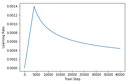
Use the Adam optimizer with a custom learning rate scheduler according to the formula in the paper.
$$\Large{lrate = d_{model}^{-0.5} min(step{_}num^{-0.5}, step{_}num warmup{_}steps^{-1.5})}$$
1 | class CustomSchedule(tf.keras.optimizers.schedules.LearningRateSchedule): |
1 | learning_rate = CustomSchedule(d_model) |
1 | temp_learning_rate_schedule = CustomSchedule(d_model) |
Text(0.5,0,'Train Step')
Loss and metrics
Since the target sequences are padded, it is important to apply a padding mask when calculating the loss.
1 | loss_object = tf.keras.losses.SparseCategoricalCrossentropy( |
1 | def loss_function(real, pred): |
1 | train_loss = tf.keras.metrics.Mean(name='train_loss') |
Training and checkpointing
1 | transformer = Transformer(num_layers, d_model, num_heads, dff, |
1 | def create_masks(inp, tar): |
Create the checkpoint path and the checkpoint manager. This will be used to save checkpoints every n epochs.
1 | checkpoint_path = "./model/transformer/checkpoints/train" |
The target is divided into tar_inp and tar_real. tar_inp is passed as an input to the decoder. tar_real is that same input shifted by 1: At each location in tar_input, tar_real contains the next token that should be predicted.
SOS=start of sentence, EOS=end of sentence
For example, sentence = “SOS A lion in the jungle is sleeping EOS”
tar_inp = “SOS A lion in the jungle is sleeping”
tar_real = “A lion in the jungle is sleeping EOS”
The transformer is an auto-regressive model: it makes predictions one part at a time, and uses its output so far to decide what to do next.
注意teacher-forcing的概念,在train的时候用real label传给下一个step。
During training this example uses teacher-forcing (like in the text generation tutorial). Teacher forcing is passing the true output to the next time step regardless of what the model predicts at the current time step.
As the transformer predicts each word, self-attention allows it to look at the previous words in the input sequence to better predict the next word.
To prevent the model from peaking at the expected output the model uses a look-ahead mask.
1 | EPOCHS = 20 |
1 |
|
Portuguese is used as the input language and English is the target language.
1 | for epoch in range(EPOCHS): |
Epoch 1 Batch 0 Loss 10.9017 Accuracy 0.0000
Epoch 1 Batch 500 Loss 4.0922 Accuracy 0.0294
Epoch 1 Loss 3.7079 Accuracy 0.0443
Time taken for 1 epoch: 110.26966953277588 secs

Epoch 2 Batch 0 Loss 2.5675 Accuracy 0.0855
Epoch 2 Batch 500 Loss 2.3795 Accuracy 0.1250
Epoch 2 Loss 2.3093 Accuracy 0.1324
Time taken for 1 epoch: 82.4690248966217 secs

Epoch 3 Batch 0 Loss 2.0194 Accuracy 0.1517
Epoch 3 Batch 500 Loss 1.9885 Accuracy 0.1704
Epoch 3 Loss 1.9433 Accuracy 0.1747
Time taken for 1 epoch: 84.78626227378845 secs

Epoch 4 Batch 0 Loss 1.7177 Accuracy 0.1863
Epoch 4 Batch 500 Loss 1.7245 Accuracy 0.1992
Epoch 4 Loss 1.6884 Accuracy 0.2023
Time taken for 1 epoch: 83.60331654548645 secs

Epoch 5 Batch 0 Loss 1.5059 Accuracy 0.2113
Epoch 5 Batch 500 Loss 1.5126 Accuracy 0.2209
Saving checkpoint for epoch 5 at ./model/transformer/checkpoints/train/ckpt-1
Epoch 5 Loss 1.4843 Accuracy 0.2230
Time taken for 1 epoch: 83.2209415435791 secs

Epoch 6 Batch 0 Loss 1.3257 Accuracy 0.2278
Epoch 6 Batch 500 Loss 1.3507 Accuracy 0.2370
Epoch 6 Loss 1.3275 Accuracy 0.2390
Time taken for 1 epoch: 79.70339369773865 secs

Epoch 7 Batch 0 Loss 1.2014 Accuracy 0.2451
Epoch 7 Batch 500 Loss 1.1911 Accuracy 0.2556
Epoch 7 Loss 1.1679 Accuracy 0.2577
Time taken for 1 epoch: 80.37797617912292 secs

Epoch 8 Batch 0 Loss 1.0367 Accuracy 0.2751
Epoch 8 Batch 500 Loss 1.0560 Accuracy 0.2726
Epoch 8 Loss 1.0396 Accuracy 0.2739
Time taken for 1 epoch: 84.6077356338501 secs

Epoch 9 Batch 0 Loss 0.9316 Accuracy 0.2829
Epoch 9 Batch 500 Loss 0.9606 Accuracy 0.2844
Epoch 9 Loss 0.9490 Accuracy 0.2852
Time taken for 1 epoch: 84.28984260559082 secs

Epoch 10 Batch 0 Loss 0.8716 Accuracy 0.2862
Epoch 10 Batch 500 Loss 0.8863 Accuracy 0.2937
Saving checkpoint for epoch 10 at ./model/transformer/checkpoints/train/ckpt-2
Epoch 10 Loss 0.8778 Accuracy 0.2942
Time taken for 1 epoch: 85.24914264678955 secs

Epoch 11 Batch 0 Loss 0.8273 Accuracy 0.2915
Epoch 11 Batch 500 Loss 0.8279 Accuracy 0.3018
Epoch 11 Loss 0.8208 Accuracy 0.3021
Time taken for 1 epoch: 84.971688747406 secs

Epoch 12 Batch 0 Loss 0.7629 Accuracy 0.3059
Epoch 12 Batch 500 Loss 0.7773 Accuracy 0.3086
Epoch 12 Loss 0.7714 Accuracy 0.3089
Time taken for 1 epoch: 84.43891286849976 secs

Epoch 13 Batch 0 Loss 0.7163 Accuracy 0.3063
Epoch 13 Batch 500 Loss 0.7394 Accuracy 0.3136
Epoch 13 Loss 0.7331 Accuracy 0.3139
Time taken for 1 epoch: 84.75990414619446 secs

Epoch 14 Batch 0 Loss 0.6871 Accuracy 0.3133
Epoch 14 Batch 500 Loss 0.7013 Accuracy 0.3190
Epoch 14 Loss 0.6963 Accuracy 0.3191
Time taken for 1 epoch: 85.32253313064575 secs

Epoch 15 Batch 0 Loss 0.6414 Accuracy 0.3162
Epoch 15 Batch 500 Loss 0.6717 Accuracy 0.3235
Saving checkpoint for epoch 15 at ./model/transformer/checkpoints/train/ckpt-3
Epoch 15 Loss 0.6675 Accuracy 0.3235
Time taken for 1 epoch: 84.33578681945801 secs

Epoch 16 Batch 0 Loss 0.6201 Accuracy 0.3232
Epoch 16 Batch 500 Loss 0.6434 Accuracy 0.3278
Epoch 16 Loss 0.6397 Accuracy 0.3277
Time taken for 1 epoch: 82.0535318851471 secs

Epoch 17 Batch 0 Loss 0.5928 Accuracy 0.3298
Epoch 17 Batch 500 Loss 0.6186 Accuracy 0.3315
Epoch 17 Loss 0.6156 Accuracy 0.3312
Time taken for 1 epoch: 86.0015115737915 secs

Epoch 18 Batch 0 Loss 0.5472 Accuracy 0.3343
Epoch 18 Batch 500 Loss 0.5961 Accuracy 0.3348
Epoch 18 Loss 0.5929 Accuracy 0.3346
Time taken for 1 epoch: 85.77375030517578 secs

Epoch 19 Batch 0 Loss 0.5477 Accuracy 0.3343
Epoch 19 Batch 500 Loss 0.5746 Accuracy 0.3385
Epoch 19 Loss 0.5726 Accuracy 0.3379
Time taken for 1 epoch: 86.64751982688904 secs

Epoch 20 Batch 0 Loss 0.5593 Accuracy 0.3331
Epoch 20 Batch 500 Loss 0.5569 Accuracy 0.3414
Saving checkpoint for epoch 20 at ./model/transformer/checkpoints/train/ckpt-4
Epoch 20 Loss 0.5543 Accuracy 0.3410
Time taken for 1 epoch: 82.36839008331299 secs
Training finished
Evaluate
The following steps are used for evaluation:
- Encode the input sentence using the Portuguese tokenizer (
tokenizer_pt). Moreover, add the start and end token so the input is equivalent to what the model is trained with. This is the encoder input. - The decoder input is the
start token == tokenizer_en.vocab_size. - Calculate the padding masks and the look ahead masks.
- The
decoderthen outputs the predictions by looking at theencoder outputand its own output (self-attention). - Select the last word and calculate the argmax of that.
- Concatentate the predicted word to the decoder input as pass it to the decoder.
- In this approach, the decoder predicts the next word based on the previous words it predicted.
Note: The model used here has less capacity to keep the example relatively faster so the predictions maybe less right. To reproduce the results in the paper, use the entire dataset and base transformer model or transformer XL, by changing the hyperparameters above.
1 | def evaluate(inp_sentence): |
1 | def plot_attention_weights(attention, sentence, result, layer): |
1 | def translate(sentence, plot=''): |
1 | translate("este é um problema que temos que resolver.") |
Input: este é um problema que temos que resolver.
Predicted translation: this is a problem that we have to solve for.com .
Real translation: this is a problem we have to solve .
1 | translate("os meus vizinhos ouviram sobre esta ideia.") |
Input: os meus vizinhos ouviram sobre esta ideia.
Predicted translation: my neighbors heard about this idea .
Real translation: and my neighboring homes heard about this idea .
1 | translate("vou então muito rapidamente partilhar convosco algumas histórias de algumas coisas mágicas que aconteceram.") |
Input: vou então muito rapidamente partilhar convosco algumas histórias de algumas coisas mágicas que aconteceram.
Predicted translation: so i 'm going to share a lot of little bit with you a few things that happened .
Real translation: so i 'll just share with you some stories very quickly of some magical things that have happened .
You can pass different layers and attention blocks of the decoder to the plot parameter.
1 | translate("este é o primeiro livro que eu fiz.", plot='decoder_layer4_block2') |
Input: este é o primeiro livro que eu fiz.
Predicted translation: this is the first book i made .
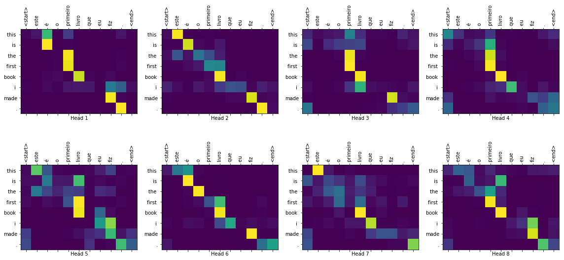
Real translation: this is the first book i've ever done.
Summary
In this tutorial, you learned about positional encoding, multi-head attention, the importance of masking and how to create a transformer.
Try using a different dataset to train the transformer. You can also create the base transformer or transformer XL by changing the hyperparameters above. You can also use the layers defined here to create BERT and train state of the art models. Futhermore, you can implement beam search to get better predictions.