Variational Autoencoder

In this assignment, you will build Variational Autoencoder, train it on the MNIST dataset, and play with its architecture and hyperparameters.

Installation

You will need

1
2
3
4
5
6
7
8
9
10
11
12
13
14
15

```python
import tensorflow as tf
import keras
import numpy as np
import matplotlib.pyplot as plt

from keras.layers import Input, Dense, Lambda, InputLayer, concatenate
from keras.models import Model, Sequential
from keras import backend as K
from keras import metrics
from keras.datasets import mnist
from keras.utils import np_utils
from grader import Grader

Grading

We will create a grader instance below and use it to collect your answers. Note that these outputs will be stored locally inside grader and will be uploaded to the platform only after running submit function in the last part of this assignment. If you want to make a partial submission, you can run that cell anytime you want.

1

grader = Grader()

Variational Autoencoder

Recall that Variational Autoencoder is a probabilistic model of data based on a continious mixture of distributions. In the lecture we covered the mixture of gaussians case, but here we will apply VAE to binary MNIST images (each pixel is either black or white). To better model binary data we will use a continuous mixture of binomial distributions(正常情况下是continuous mixture of gaussian distribution. 表达式一样，主要体现在reconstruction error 上): $p(x \mid w) = \int p(x \mid t, w) p(t) dt$, where the prior distribution on the latent code $t$ is standard normal $p(t) = \mathcal{N}(0, I)$, but probability that $(i, j)$-th pixel is black equals to $(i, j)$-th output of the decoder neural detwork: $p(x_{i, j} \mid t, w) = \text{decoder}(t, w)_{i, j}$.

To train this model we would like to maximize marginal log-likelihood of our dataset $\max_w \log p(X \mid w)$, but it’s very hard to do computationally, so instead we maximize the Variational Lower Bound w.r.t. both the original parameters $w$ and variational distribution $q$ which we define as encoder neural network with parameters $\phi$ which takes input image $x$ and outputs parameters of the gaussian distribution $q(t \mid x, \phi)$: $\log p(X \mid w) \geq \mathcal{L}(w, \phi) \rightarrow \max_{w, \phi}$.

注意：这里有三个概念：likelihood, prior 和 variational. Likelihood是$p(X \mid w)$，即我们最后要maximize的。Prior是standard normal $p(t) = \mathcal{N}(0, I)$。Posterior即$p(t \mid x)$。 Variance是我们用encoder模拟的Prior即$q(t \mid x, \phi)$

So overall our model looks as follows: encoder takes an image $x$, produces a distribution over latent codes $q(t \mid x)$ which should approximate the posterior distribution $p(t \mid x)$ (at least after training), samples a point from this distribution $\widehat{t} \sim q(t \mid x, \phi)$, and finally feeds it into a decoder that outputs a distribution over images.

In the lecture, we also discussed that variational lower bound has an expected value inside which we are going to approximate with sampling. But it is not trivial since we need to differentiate through this approximation. However, we learned about reparametrization trick which suggests instead of sampling from distribution $\widehat{t} \sim q(t \mid x, \phi)$ sample from a distribution which doesn’t depend on any parameters, e.g. standard normal, and then deterministically transform this sample to the desired one: $\varepsilon \sim \mathcal{N}(0, I); ~~\widehat{t} = m(x, \phi) + \varepsilon \sigma(x, \phi)$. This way we don’t have to worry about our stochastic gradient being biased and can straightforwardly differentiate our loss w.r.t. all the parameters while treating the current sample $\varepsilon$ as constant.

Variational Lower Bound

Task 1 Derive and implement Variational Lower Bound for the continuous mixture of Binomial distributions.

Note that to pass the test, your code should work with any mini-batch size.

Also note that although we need a stochastic estimate of VLB:
$$\text{VLB} = \sum_{i=1}^N \text{VLB}i \approx \frac{N}{M}\sum{i_s}^M \text{VLB}_{i_s}$$
where $N$ is the dataset size, $\text{VLB}i$ is the term of VLB corresponding to the $i$-th object, and $M$ is the mini-batch size; in the function below you need to return just average across the mini-batch $\frac{1}{M}\sum{i_s}^M \text{VLB}_{i_s}$. People usually optimize this unscaled version of VLB since it doesn’t depend on the dataset set size - you can write VLB function once and use it for different datasets - and it doesn’t affect optimization (it does affect the learning rate though). The correct value for this unscaled VLB should be around $100 - 170$.

1
2
3
4
5
6
7
8
9
10
11
12
13
14
15
16
17
18
19
20
21

def vlb_binomial(x, x_decoded_mean, t_mean, t_log_var):
    """Returns the value of Variational Lower Bound
    
    The inputs are tf.Tensor
        x: (batch_size x number_of_pixels) matrix with one image per row with zeros and ones
        x_decoded_mean: (batch_size x number_of_pixels) mean of the distribution p(x | t), real numbers from 0 to 1
        t_mean: (batch_size x latent_dim) mean vector of the (normal) distribution q(t | x)
        t_log_var: (batch_size x latent_dim) logarithm of the variance vector of the (normal) distribution q(t | x)
    
    Returns:
        A tf.Tensor with one element (averaged across the batch), VLB
    """
    ### YOUR CODE HERE
    ## vlb is the loss function, having reconstruction error and kl divergence
    ## kl divergence is KL(q||p), w.r.t q is estimated Gaussian, p is Normal Gaussian
    kl = tf.reduce_sum((tf.exp(t_log_var) + t_mean**2 - t_log_var - 1)/2, 1)
    ## reconstruction loss uses cross entropy, since it's binary image
    reconstruction_loss = -tf.reduce_sum(x*tf.log(x_decoded_mean+1e-8)+(1-x)*tf.log(1-x_decoded_mean+1e-8), 1)
    kl = tf.reduce_mean(kl)
    reconstruction_loss = tf.reduce_mean(reconstruction_loss)
    return reconstruction_loss + kl

1
2
3
4

# Start tf session so we can run code.
sess = tf.InteractiveSession()
# Connect keras to the created session.
K.set_session(sess)

1

grader.submit_vlb(sess, vlb_binomial)

Current answer for task 1 (vlb) is: 157.59695

Encoder / decoder definition

Task 2 Read the code below that defines encoder and decoder networks and implement sampling with reparametrization trick in the provided space.

1
2
3
4
5
6
7
8
9
10
11
12
13
14
15
16
17
18
19
20
21
22
23
24
25
26
27
28
29
30
31
32
33
34
35
36
37
38
39
40
41
42
43
44
45
46
47
48
49
50
51
52
53
54
55
56
57
58

batch_size = 100
original_dim = 784 # Number of pixels in MNIST images.
latent_dim = 64 # d, dimensionality of the latent code t.
intermediate_dim = 256 # Size of the hidden layer.
epochs = 40

x = Input(batch_shape=(batch_size, original_dim))
def create_encoder(input_dim):
    # Encoder network.
    # We instantiate these layers separately so as to reuse them later
    encoder = Sequential(name='encoder')
    encoder.add(InputLayer([input_dim]))
    encoder.add(Dense(intermediate_dim, activation='relu'))
    encoder.add(Dense(2 * latent_dim))
    return encoder
encoder = create_encoder(original_dim)

get_t_mean = Lambda(lambda h: h[:, :latent_dim])
get_t_log_var = Lambda(lambda h: h[:, latent_dim:])
h = encoder(x)
t_mean = get_t_mean(h)
t_log_var = get_t_log_var(h)

# Sampling from the distribution 
#     q(t | x) = N(t_mean, exp(t_log_var))
# with reparametrization trick.
def sampling(args):
    """Returns sample from a distribution N(args[0], diag(args[1]))
    
    The sample should be computed with reparametrization trick.
    
    The inputs are tf.Tensor
        args[0]: (batch_size x latent_dim) mean of the desired distribution
        args[1]: (batch_size x latent_dim) logarithm of the variance vector of the desired distribution
    
    Returns:
        A tf.Tensor of size (batch_size x latent_dim), the samples.
    """
    t_mean, t_log_var = args
    # YOUR CODE HERE
    ## Use reparametrization trick
    epsilon = tf.random_normal(t_mean.shape)
    z = epsilon * tf.exp(0.5 * t_log_var) + t_mean
    return z


t = Lambda(sampling)([t_mean, t_log_var])

def create_decoder(input_dim):
    # Decoder network
    # We instantiate these layers separately so as to reuse them later
    decoder = Sequential(name='decoder')
    decoder.add(InputLayer([input_dim]))
    decoder.add(Dense(intermediate_dim, activation='relu'))
    decoder.add(Dense(original_dim, activation='sigmoid'))
    return decoder
decoder = create_decoder(latent_dim)
x_decoded_mean = decoder(t)

1

grader.submit_samples(sess, sampling)

Current answer for task 2.1 (samples mean) is: -0.118285365
Current answer for task 2.2 (samples var) is: 0.03759662

Training the model

Task 3 Run the cells below to train the model with the default settings. Modify the parameters to get better results. Especially pay attention the encoder / encoder architectures (e.g. using more layers, maybe making them convolutional), learning rate, and the number of epochs.

1
2
3
4
5
6
7
8

# Note here the lower bound defined before is actually loss (- lower_bound)
loss = vlb_binomial(x, x_decoded_mean, t_mean, t_log_var)
vae = Model(x, x_decoded_mean)
# Keras will provide input (x) and output (x_decoded_mean) to the function that
# should construct loss, but since our function also depends on other
# things (e.g. t_means), it is easier to build the loss in advance and pass
# a function that always returns it.
vae.compile(optimizer=keras.optimizers.RMSprop(lr=0.001), loss=lambda x, y: loss)

Load and prepare the data

1
2

# train the VAE on MNIST digits
(x_train, y_train), (x_test, y_test) = mnist.load_data()

1
2
3
4
5
6
7
8
9
10
11
12

# One hot encoding.
## y_train, y_test is class of the image, 0~9. Not used for VAE, used for CVAE
y_train = np_utils.to_categorical(y_train)
y_test = np_utils.to_categorical(y_test)

## change binary image to continuous input 0~1
x_train = x_train.astype('float32') / 255.
x_test = x_test.astype('float32') / 255.

## flatten x_train and x_test
x_train = x_train.reshape((len(x_train), np.prod(x_train.shape[1:])))
x_test = x_test.reshape((len(x_test), np.prod(x_test.shape[1:])))

Train the model

1
2
3
4
5
6

hist = vae.fit(x=x_train, y=x_train,
               shuffle=True,
               epochs=epochs,
               batch_size=batch_size,
               validation_data=(x_test, x_test),
               verbose=2)

Train on 60000 samples, validate on 10000 samples
Epoch 1/40
 - 4s - loss: 162.7900 - val_loss: 138.6159
Epoch 2/40
 - 3s - loss: 131.5424 - val_loss: 124.2565
Epoch 3/40
 - 3s - loss: 122.4806 - val_loss: 118.1873
Epoch 4/40
 - 3s - loss: 117.4147 - val_loss: 115.3841
Epoch 5/40
 - 3s - loss: 114.3555 - val_loss: 112.6461
Epoch 6/40
 - 3s - loss: 112.4335 - val_loss: 110.8228
Epoch 7/40
 - 3s - loss: 111.1243 - val_loss: 109.4895
Epoch 8/40
 - 3s - loss: 110.1543 - val_loss: 109.0790
Epoch 9/40
 - 3s - loss: 109.5377 - val_loss: 108.8097
Epoch 10/40
 - 3s - loss: 109.0028 - val_loss: 108.1919
Epoch 11/40
 - 3s - loss: 108.6090 - val_loss: 108.2727
Epoch 12/40
 - 3s - loss: 108.2288 - val_loss: 108.0635
Epoch 13/40
 - 3s - loss: 107.9554 - val_loss: 107.1368
Epoch 14/40
 - 3s - loss: 107.6794 - val_loss: 107.2797
Epoch 15/40
 - 3s - loss: 107.4163 - val_loss: 107.0116
Epoch 16/40
 - 3s - loss: 107.2714 - val_loss: 106.8392
Epoch 17/40
 - 3s - loss: 107.0786 - val_loss: 106.5130
Epoch 18/40
 - 3s - loss: 106.9363 - val_loss: 106.5109
Epoch 19/40
 - 3s - loss: 106.7659 - val_loss: 106.8130
Epoch 20/40
 - 3s - loss: 106.6219 - val_loss: 105.9736
Epoch 21/40
 - 3s - loss: 106.5032 - val_loss: 106.2564
Epoch 22/40
 - 3s - loss: 106.4050 - val_loss: 106.0565
Epoch 23/40
 - 3s - loss: 106.3155 - val_loss: 107.0727
Epoch 24/40
 - 3s - loss: 106.1915 - val_loss: 106.0746
Epoch 25/40
 - 3s - loss: 106.0905 - val_loss: 105.9534
Epoch 26/40
 - 3s - loss: 106.0185 - val_loss: 105.7398
Epoch 27/40
 - 3s - loss: 105.9506 - val_loss: 106.0413
Epoch 28/40
 - 3s - loss: 105.8656 - val_loss: 105.6316
Epoch 29/40
 - 3s - loss: 105.7916 - val_loss: 104.9242
Epoch 30/40
 - 3s - loss: 105.6715 - val_loss: 105.2510
Epoch 31/40
 - 3s - loss: 105.6575 - val_loss: 105.2133
Epoch 32/40
 - 3s - loss: 105.5556 - val_loss: 104.6787
Epoch 33/40
 - 3s - loss: 105.4921 - val_loss: 104.8313
Epoch 34/40
 - 3s - loss: 105.4479 - val_loss: 105.3083
Epoch 35/40
 - 3s - loss: 105.3896 - val_loss: 105.2446
Epoch 36/40
 - 3s - loss: 105.3886 - val_loss: 104.5037
Epoch 37/40
 - 3s - loss: 105.2930 - val_loss: 105.2558
Epoch 38/40
 - 3s - loss: 105.2345 - val_loss: 104.9638
Epoch 39/40
 - 3s - loss: 105.2255 - val_loss: 104.9504
Epoch 40/40
 - 3s - loss: 105.1552 - val_loss: 104.8775

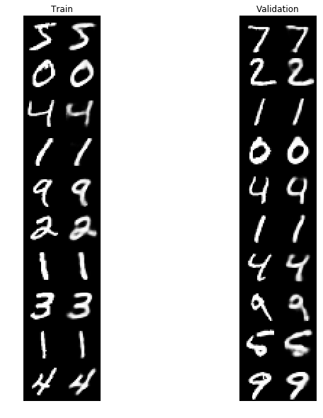
Visualize reconstructions for train and validation data

In the picture below you can see the reconstruction ability of your network on training and validation data. In each of the two images, the left column is MNIST images and the right column is the corresponding image after passing through autoencoder (or more precisely the mean of the binomial distribution over the output images).

Note that getting the best possible reconstruction is not the point of VAE, the KL term of the objective specifically hurts the reconstruction performance. But the reconstruction should be anyway reasonable and they provide a visual debugging tool.

1
2
3
4
5
6
7
8
9
10
11
12
13
14
15
16
17

fig = plt.figure(figsize=(10, 10))
for fid_idx, (data, title) in enumerate(
            zip([x_train, x_test], ['Train', 'Validation'])):
    n = 10  # figure with 10 x 2 digits
    digit_size = 28
    figure = np.zeros((digit_size * n, digit_size * 2))
    decoded = sess.run(x_decoded_mean, feed_dict={x: data[:batch_size, :]})
    for i in range(10):
        figure[i * digit_size: (i + 1) * digit_size,
               :digit_size] = data[i, :].reshape(digit_size, digit_size)
        figure[i * digit_size: (i + 1) * digit_size,
               digit_size:] = decoded[i, :].reshape(digit_size, digit_size)
    ax = fig.add_subplot(1, 2, fid_idx + 1)
    ax.imshow(figure, cmap='Greys_r')
    ax.set_title(title)
    ax.axis('off')
plt.show()

Sending the results of your best model as Task 3 submission

1

grader.submit_best_val_loss(hist)

Current answer for task 3 (best val loss) is: 104.87750022888184

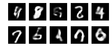
Hallucinating new data

Task 4 Write code to generate new samples of images from your trained VAE. To do that you have to sample from the prior distribution $p(t)$ and then from the likelihood $p(x \mid t)$.

Note that the sampling you’ve written in Task 2 was for the variational distribution $q(t \mid x)$, while here you need to sample from the prior.

这里注意！sample是从prior sample，而prior sample是 Normal Gaussian

1
2
3
4
5
6
7

n_samples = 10  # To pass automatic grading please use at least 2 samples here.
# YOUR CODE HERE.

# sampled_im_mean is a tf.Tensor of size 10 x 784 with 10 random
# images sampled from the vae model.
z = tf.random_normal((n_samples, latent_dim))
sampled_im_mean = decoder(z)

1
2
3
4
5
6
7
8

sampled_im_mean_np = sess.run(sampled_im_mean)
# Show the sampled images.
plt.figure()
for i in range(n_samples):
    ax = plt.subplot(n_samples // 5 + 1, 5, i + 1)
    plt.imshow(sampled_im_mean_np[i, :].reshape(28, 28), cmap='gray')
    ax.axis('off')
plt.show()

1

grader.submit_hallucinating(sess, sampled_im_mean)

Current answer for task 4.1 (hallucinating mean) is: 0.10742197
Current answer for task 4.2 (hallucinating var) is: 0.18451297

Conditional VAE

In the final task, you will modify your code to obtain Conditional Variational Autoencoder [1]. The idea is very simple: to be able to control the samples you generate, we condition all the distributions on some additional information. In our case, this additional information will be the class label (the digit on the image, from 0 to 9).

So now both the likelihood and the variational distributions are conditioned on the class label: $p(x \mid t, \text{label}, w)$, $q(t \mid x, \text{label}, \phi)$.

The only thing you have to change in your code is to concatenate input image $x$ with (one-hot) label of this image to pass into the encoder $q$ and to concatenate latent code $t$ with the same label to pass into the decoder $p$. Note that it’s slightly harder to do with convolutional encoder / decoder model.

[1] Sohn, Kihyuk, Honglak Lee, and Xinchen Yan. “Learning Structured Output Representation using Deep Conditional Generative Models.” Advances in Neural Information Processing Systems. 2015.

Final task

Task 5.1 Implement CVAE model. You may reuse

1
2
3
4
5
6
7
8
9
10
11
12
13
14
15
16
17
18
19
20
21
22
23

To finish this task, you should go to `Conditionally hallucinate data` section and find there Task 5.2


```python
# One-hot labels placeholder.
x = Input(batch_shape=(batch_size, original_dim))
label = Input(batch_shape=(batch_size, 10))

# YOUR CODE HERE
cond_encoder = create_encoder(original_dim + 10)

# get_t_mean = Lambda(lambda h: h[:, :latent_dim])
# get_t_log_var = Lambda(lambda h: h[:, latent_dim:])
cond_h = cond_encoder(concatenate([x, label]))
cond_t_mean = get_t_mean(cond_h)
cond_t_log_var = get_t_log_var(cond_h)


t = Lambda(sampling)([cond_t_mean, cond_t_log_var])

cond_decoder = create_decoder(latent_dim + 10)
cond_x_decoded_mean = cond_decoder(concatenate([t, label]))

Define the loss and the model

1
2
3

conditional_loss = vlb_binomial(x, cond_x_decoded_mean, cond_t_mean, cond_t_log_var)
cvae = Model([x, label], cond_x_decoded_mean)
cvae.compile(optimizer=keras.optimizers.RMSprop(lr=0.001), loss=lambda x, y: conditional_loss)

Train the model

1
2
3
4
5
6
7

hist = cvae.fit(x=[x_train, y_train],
                y=x_train,
                shuffle=True,
                epochs=epochs,
                batch_size=batch_size,
                validation_data=([x_test, y_test], x_test),
                verbose=2)

Train on 60000 samples, validate on 10000 samples
Epoch 1/40
 - 4s - loss: 160.0676 - val_loss: 133.8433
Epoch 2/40
 - 4s - loss: 128.0758 - val_loss: 122.0311
Epoch 3/40
 - 4s - loss: 118.6988 - val_loss: 115.4986
Epoch 4/40
 - 4s - loss: 113.6957 - val_loss: 110.6210
Epoch 5/40
 - 4s - loss: 110.7541 - val_loss: 109.4086
Epoch 6/40
 - 4s - loss: 108.8539 - val_loss: 106.9255
Epoch 7/40
 - 4s - loss: 107.4996 - val_loss: 105.8797
Epoch 8/40
 - 4s - loss: 106.6003 - val_loss: 105.6026
Epoch 9/40
 - 4s - loss: 105.7587 - val_loss: 106.0383
Epoch 10/40
 - 4s - loss: 105.1994 - val_loss: 105.1134
Epoch 11/40
 - 4s - loss: 104.7207 - val_loss: 103.5558
Epoch 12/40
 - 4s - loss: 104.2589 - val_loss: 103.2119
Epoch 13/40
 - 4s - loss: 103.9110 - val_loss: 103.2548
Epoch 14/40
 - 4s - loss: 103.5644 - val_loss: 102.4616
Epoch 15/40
 - 4s - loss: 103.2869 - val_loss: 103.0862
Epoch 16/40
 - 4s - loss: 103.0542 - val_loss: 102.2632
Epoch 17/40
 - 4s - loss: 102.8694 - val_loss: 102.1227
Epoch 18/40
 - 4s - loss: 102.6723 - val_loss: 102.1841
Epoch 19/40
 - 4s - loss: 102.4552 - val_loss: 101.9109
Epoch 20/40
 - 4s - loss: 102.3108 - val_loss: 102.6435
Epoch 21/40
 - 4s - loss: 102.1548 - val_loss: 102.3394
Epoch 22/40
 - 4s - loss: 101.9564 - val_loss: 101.4016
Epoch 23/40
 - 4s - loss: 101.8731 - val_loss: 102.0562
Epoch 24/40
 - 4s - loss: 101.7377 - val_loss: 102.8159
Epoch 25/40
 - 4s - loss: 101.6051 - val_loss: 101.0873
Epoch 26/40
 - 4s - loss: 101.5291 - val_loss: 100.6189
Epoch 27/40
 - 4s - loss: 101.3765 - val_loss: 101.9504
Epoch 28/40
 - 4s - loss: 101.3285 - val_loss: 101.1729
Epoch 29/40
 - 4s - loss: 101.1974 - val_loss: 101.2699
Epoch 30/40
 - 4s - loss: 101.0955 - val_loss: 101.3118
Epoch 31/40
 - 4s - loss: 100.9785 - val_loss: 101.4562
Epoch 32/40
 - 4s - loss: 100.9389 - val_loss: 100.6755
Epoch 33/40
 - 4s - loss: 100.8765 - val_loss: 100.1449
Epoch 34/40
 - 4s - loss: 100.7750 - val_loss: 102.4070
Epoch 35/40
 - 4s - loss: 100.7393 - val_loss: 100.7936
Epoch 36/40
 - 4s - loss: 100.6984 - val_loss: 100.2737
Epoch 37/40
 - 4s - loss: 100.6426 - val_loss: 100.4940
Epoch 38/40
 - 4s - loss: 100.5590 - val_loss: 100.5555
Epoch 39/40
 - 4s - loss: 100.4930 - val_loss: 100.2847
Epoch 40/40
 - 4s - loss: 100.4308 - val_loss: 100.0369

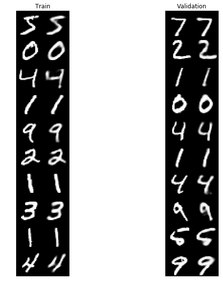
Visualize reconstructions for train and validation data

1
2
3
4
5
6
7
8
9
10
11
12
13
14
15
16
17
18
19

fig = plt.figure(figsize=(10, 10))
for fid_idx, (x_data, y_data, title) in enumerate(
            zip([x_train, x_test], [y_train, y_test], ['Train', 'Validation'])):
    n = 10  # figure with 10 x 2 digits
    digit_size = 28
    figure = np.zeros((digit_size * n, digit_size * 2))
    decoded = sess.run(cond_x_decoded_mean,
                       feed_dict={x: x_data[:batch_size, :],
                                  label: y_data[:batch_size, :]})
    for i in range(10):
        figure[i * digit_size: (i + 1) * digit_size,
               :digit_size] = x_data[i, :].reshape(digit_size, digit_size)
        figure[i * digit_size: (i + 1) * digit_size,
               digit_size:] = decoded[i, :].reshape(digit_size, digit_size)
    ax = fig.add_subplot(1, 2, fid_idx + 1)
    ax.imshow(figure, cmap='Greys_r')
    ax.set_title(title)
    ax.axis('off')
plt.show()

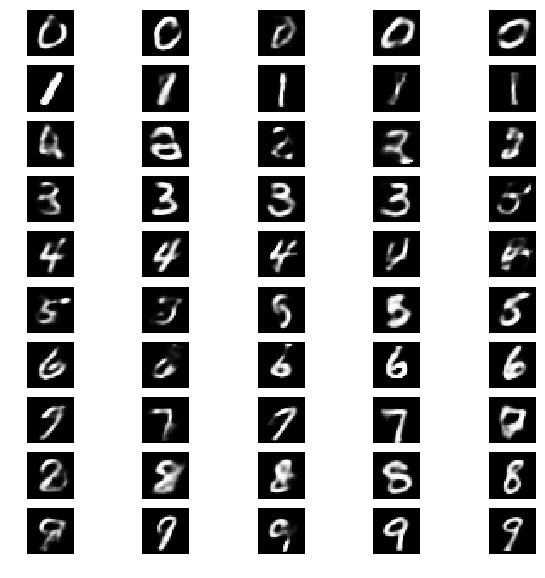
Conditionally hallucinate data

Task 5.2 Implement the conditional sampling from the distribution $p(x \mid t, \text{label})$ by firstly sampling from the prior $p(t)$ and then sampling from the likelihood $p(x \mid t, \text{label})$.

1
2
3
4
5
6
7
8
9
10
11
12

# Prepare one hot labels of form
#   0 0 0 0 0 1 1 1 1 1 2 2 2 2 2 ...
# to sample five zeros, five ones, etc
curr_labels = np.eye(10)
curr_labels = np.repeat(curr_labels, 5, axis=0)  # Its shape is 50 x 10.
# YOUR CODE HERE.
# ...
# cond_sampled_im_mean is a tf.Tensor of size 50 x 784 with 5 random zeros,
# then 5 random ones, etc sampled from the cvae model.
tensor_labels=tf.convert_to_tensor(curr_labels,dtype=tf.float32)
z = tf.random_normal((50, latent_dim))
cond_sampled_im_mean = cond_decoder(concatenate([z, tensor_labels]))

1
2
3
4
5
6
7
8
9
10
11

cond_sampled_im_mean_np = sess.run(cond_sampled_im_mean)
# Show the sampled images.
plt.figure(figsize=(10, 10))
global_idx = 0
for digit in range(10):
    for _ in range(5):
        ax = plt.subplot(10, 5, global_idx + 1)
        plt.imshow(cond_sampled_im_mean_np[global_idx, :].reshape(28, 28), cmap='gray')
        ax.axis('off')
        global_idx += 1
plt.show()

1
2

# Submit Task 5 (both 5.1 and 5.2).
grader.submit_conditional_hallucinating(sess, cond_sampled_im_mean)

Current answer for task 5.1 (conditional hallucinating mean) is: 0.09869497077779138
Current answer for task 5.2 (conditional hallucinating var) is: 0.04790131456509189

Authorization & Submission

To submit assignment parts to Cousera platform, please, enter your e-mail and token into variables below. You can generate the token on this programming assignment page. Note: Token expires 30 minutes after generation.

1
2
3

STUDENT_EMAIL = ''# EMAIL HERE
STUDENT_TOKEN =  '' # TOKEN HERE
grader.status()

You want to submit these numbers:
Task 1 (vlb): 157.59695
Task 2.1 (samples mean): -0.118285365
Task 2.2 (samples var): 0.03759662
Task 3 (best val loss): 104.87750022888184
Task 4.1 (hallucinating mean): 0.10742197
Task 4.2 (hallucinating var): 0.18451297
Task 5.1 (conditional hallucinating mean): 0.09869497077779138
Task 5.2 (conditional hallucinating var): 0.04790131456509189

1

grader.submit(STUDENT_EMAIL, STUDENT_TOKEN)

Submitted to Coursera platform. See results on assignment page!

Playtime (UNGRADED)

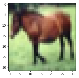
Once you passed all the tests, modify the code below to work with the mixture of Gaussian distributions (in contrast to the mixture of Binomial distributions), and redo the experiments with CIFAR-10 dataset, which are much full color natural images.

1
2

from keras.datasets import cifar10
(x_train, y_train), (x_test, y_test) = cifar10.load_data()

Downloading data from https://www.cs.toronto.edu/~kriz/cifar-10-python.tar.gz
170500096/170498071 [==============================] - 24s 0us/step

1
2

plt.imshow(x_train[7, :])
plt.show()