Gaussian processes and Bayesian optimization

In this assignment you will learn how to use GPy and GPyOpt libraries to deal with gaussian processes. These libraries provide quite simple and inuitive interfaces for training and inference, and we will try to get familiar with them in a few tasks.

Installation

New libraries that are required for this tasks can be installed with the following command (if you use Anaconda):

1
2
3

pip install GPy 
pip install gpyopt 
pip install xgboost

You can also follow installtaion guides from GPy and GPyOpt if you want to build them from source

You will also need following libraries:

1
2
3
4
5
6
7
8
9
10
11
12
13
14

```python
import numpy as np
import GPy
import GPyOpt
import matplotlib.pyplot as plt
from sklearn.svm import SVR
import sklearn.datasets
from xgboost import XGBRegressor
from sklearn.cross_validation import cross_val_score
import time
from grader import Grader
%matplotlib inline

/home/dongnanzhy/miniconda3/lib/python3.6/site-packages/sklearn/cross_validation.py:41: DeprecationWarning:This module was deprecated in version 0.18 in favor of the model_selection module into which all the refactored classes and functions are moved. Also note that the interface of the new CV iterators are different from that of this module. This module will be removed in 0.20.

Grading

We will create a grader instace below and use it to collect your answers. Note that these outputs will be stored locally inside grader and will be uploaded to platform only after running submiting function in the last part of this assignment. If you want to make partial submission, you can run that cell any time you want.

1

grader = Grader()

Gaussian processes: GPy (documentation)

We will start with a simple regression problem, for which we will try to fit a Gaussian Process with RBF kernel.

1
2
3
4
5
6
7
8
9
10
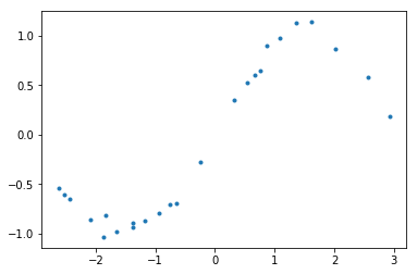
11

def generate_points(n=25, noise_variance=0.0036):
    np.random.seed(777)
    X = np.random.uniform(-3.,3.,(n,1))
    y = np.sin(X) + np.random.randn(n,1)*noise_variance**0.5
    return X, y
    
def generate_noise(n=25, noise_variance=0.0036):
    np.random.seed(777)
    X = np.random.uniform(-3.,3.,(n,1))
    y = np.random.randn(n,1)*noise_variance**0.5
    return X, y

1
2
3
4

# Create data points
X, y = generate_points()
plt.plot(X, y, '.')
plt.show()

To fit a Gaussian Process, you will need to define a kernel. For Gaussian (GBF) kernel you can use GPy.kern.RBF
function.

Task 1.1: Create RBF kernel with variance 1.5 and length-scale parameter 2 for 1D samples and compute value of the kernel between 6-th and 10-th points (one-based indexing system). Submit a single number.

Hint: use

1
2
3
4
5
6

```python
kernel = GPy.kern.RBF(input_dim=1, variance=1.5, lengthscale=2.) ### YOUR CODE HERE
kernel_59 = kernel.K(X[5].reshape(1,1),X[9].reshape(1,1)) ### YOUR CODE HERE
grader.submit_GPy_1(kernel_59)

Current answer for task 1.1 is: 1.0461813545396959

Task 1.2: Fit GP into generated data. Use kernel from previous task. Submit predicted mean and vairance at position $x=1$.

Hint: use

1
2
3
4
5
6

```python
model = GPy.models.GPRegression(X,y,kernel) ### YOUR CODE HERE
mean,variance = model.predict(np.array([[1]])) ### YOUR CODE HERE
grader.submit_GPy_2(mean, variance)

Current answer for task 1.2 (mean) is: 0.6646774926102937
Current answer for task 1.2 (variance) is: 1.1001478223790582

1
2

model.plot()
plt.show()

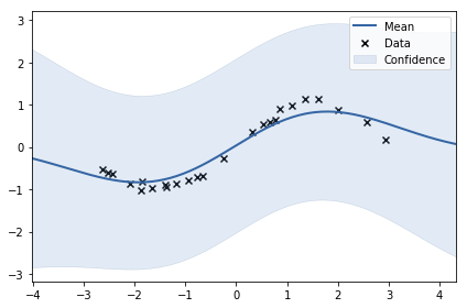
We see that model didn’t fit the data quite well. Let’s try to fit kernel and noise parameters automatically as discussed in the lecture! You can see current parameters below:

1

model

Model: GP regression

Objective: 27.86687636693494

Number of Parameters: 3

Number of Optimization Parameters: 3

Updates: True

1
2
3
4
5
6
7

```python
### YOUR CODE HERE
model.optimize()
lengthscale = kernel.lengthscale
grader.submit_GPy_3(lengthscale)

1
2

model.plot()
plt.show()

1

model

Model: GP regression

Objective: -18.351767754167483

Number of Parameters: 3

Number of Optimization Parameters: 3

Updates: True

可以看到GP自动optimize出来最初设定的gaussian noise variance

As you see, process generates outputs just right. Let’s see if GP can figure out itself when we try to fit it into noise or signal.

Task 1.4: Generate two datasets: sinusoid wihout noise and samples from gaussian noise. Optimize kernel parameters and submit optimal values of noise component.

Note: generate data only using

1
2
3
4
5
6
7
8
9
10

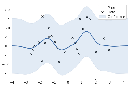
```python
X, y = generate_noise(noise_variance=10)
### YOUR CODE HERE
kernel = GPy.kern.RBF(1, 1.5, 2)
model = GPy.models.GPRegression(X,y,kernel)
model.optimize()
noise = model.Gaussian_noise.variance
model.plot()

<matplotlib.axes._subplots.AxesSubplot at 0x7f197c3657f0>

1
2
3
4
5
6
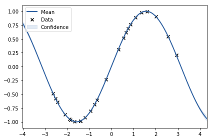
7

X, y = generate_points(noise_variance=0)
### YOUR CODE HERE
kernel = GPy.kern.RBF(1, 1.5, 2)
model = GPy.models.GPRegression(X,y,kernel)
model.optimize()
just_signal = model.Gaussian_noise.variance
model.plot()

<matplotlib.axes._subplots.AxesSubplot at 0x7f197c2ead30>

1

grader.submit_GPy_4(noise, just_signal)

Current answer for task 1.4 (noise) is: 10.143341903515504
Current answer for task 1.4 (just signal) is: 8.89286451503942e-16

Sparce GP

Now let’s consider the speed of GP. We will generate a dataset of 3000 points and measure time that is consumed for prediction of mean and variance for each point. We will then try to use indusing inputs and find optimal number of points according to quality-time tradeoff.

For sparse model with inducing points you should use

1
2
3
4
5
6

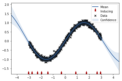
<b>Task 1.5</b>: Create a dataset of 1000 points and fit GPRegression. Measure time for predicting mean and variance at position $x=1$. Then fit SparseGPRegression with 10 inducing inputs and repeat the experiment. Report speedup as a ratio between consumed time without and with inducing inputs.


```python
X, y = generate_points(1000)

1
2
3
4
5
6
7

### YOUR CODE HERE
kernel = GPy.kern.RBF(1, 1.5, 2)
model = GPy.models.GPRegression(X,y, kernel)
model.optimize()
start = time.time()
mean, variance = model.predict(np.array([[1]]))
time_gp = time.time()-start

1
2
3
4
5
6
7

### YOUR CODE HERE
kernel = GPy.kern.RBF(1, 1.5, 2)
model = GPy.models.SparseGPRegression(X,y, kernel, num_inducing=10)
model.optimize()
start = time.time()
mean, variance = model.predict(np.array([[1]]))
time_sgp = time.time()-start

1
2

model.plot()
plt.show()

1

grader.submit_GPy_5(time_gp / time_sgp)

Current answer for task 1.5 is: 3.7309941520467835

Bayesian optimization: GPyOpt (documentation, tutorials)

In this part of the assignment we will try to find optimal hyperparameters to XGBoost model! We will use data from a small competition to speed things up, but keep in mind that the approach works even for large datasets.

We will use diabetes dataset provided in sklearn package.

1
2
3

dataset = sklearn.datasets.load_diabetes()
X = dataset['data']
y = dataset['target']

We will use cross validation score to estimate accuracy and our goal will be to tune:

1
2
3
4
5
6
7
8
9
10
11
12
13
14
15

```python
# Score. Optimizer will try to find minimum, so we will add a "-" sign.
def f(parameters):
    parameters = parameters[0]
    score = -cross_val_score(
                XGBRegressor(learning_rate=parameters[0],
                              max_depth=int(parameters[2]),
                              n_estimators=int(parameters[3]),
                              gamma=int(parameters[1]),
                              min_child_weight = parameters[4]), 
                X, y, scoring='neg_mean_squared_error').mean()
    score = np.array(score)
    return score

1
2

baseline = -cross_val_score(XGBRegressor(), X, y, scoring='neg_mean_squared_error').mean()
baseline

3498.951701204653

1
2
3
4
5
6
7
8

# Bounds (NOTE: define continuous variables first, then discrete!)
bounds = [
            {'name': 'learning_rate', 'type': 'continuous', 'domain': (0, 1)},
            {'name': 'gamma', 'type': 'continuous', 'domain': (0, 5)},
            {'name': 'max_depth', 'type': 'discrete', 'domain': (1, 50)},
            {'name': 'n_estimators', 'type': 'discrete', 'domain': (1, 300)},
            {'name': 'min_child_weight', 'type': 'discrete', 'domain': (1, 10)}
         ]

1
2
3
4
5

np.random.seed(777)
optimizer = GPyOpt.methods.BayesianOptimization(f=f, domain=bounds,
                                                acquisition_type ='MPI',
                                                acquisition_par = 0.1,
                                                exact_eval=True)

1
2
3

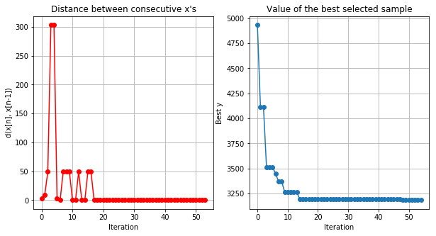
max_iter = 50
max_time = 60
optimizer.run_optimization(max_iter, max_time)

1

optimizer.plot_convergence()

Best values of parameters:

1

optimizer.X[np.argmin(optimizer.Y)]

array([7.69938334e-02, 1.20414169e+00, 1.00000000e+00, 3.00000000e+02,
       1.00000000e+00])

1

print('MSE:', np.min(optimizer.Y), 'Gain:', baseline/np.min(optimizer.Y)*100)

MSE: 3184.586757459207 Gain: 109.87145170434167

We were able to get 9% boost wihtout tuning parameters by hand! Let’s see if you can do the same.

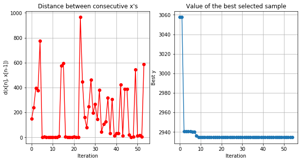
Task 2.1: Tune SVR model. Find optimal values for three parameters:

1
2
3
4
5

```python
baseline = -cross_val_score(SVR(), X, y, scoring='neg_mean_squared_error').mean()
baseline

6067.652263997995

1
2
3
4
5
6
7
8
9
10
11
12
13
14
15
16
17
18
19
20
21
22
23
24
25

def f(parameters):
    parameters = parameters[0]
    score = -cross_val_score(
                SVR(C=parameters[0],
                    epsilon=parameters[2],
                    gamma=parameters[1]), 
                X, y, scoring='neg_mean_squared_error').mean()
    score = np.array(score)
    return score
        
bounds = [
            {'name': 'C', 'type': 'continuous', 'domain': (1e-5, 1000)},
            {'name': 'gamma', 'type': 'continuous', 'domain': (1e-5, 10)},
            {'name': 'epsilon', 'type': 'continuous', 'domain': (1e-5, 10)}
         ]
        
np.random.seed(777)
optimizer = GPyOpt.methods.BayesianOptimization(f=f, domain=bounds,
                                                acquisition_type ='MPI',
                                                acquisition_par = 0.1,
                                                exact_eval=True)

max_iter = 50
max_time = 60
optimizer.run_optimization(max_iter, max_time)

1

optimizer.plot_convergence()

1
2
3

### YOUR CODE HERE
best_epsilon = optimizer.X[np.argmin(optimizer.Y)][2]### YOUR CODE HERE
grader.submit_GPyOpt_1(best_epsilon)

Current answer for task 2.1 is: 10.0

Task 2.2: For the model above submit boost in improvement that you got after tuning hyperparameters (output percents) [e.g. if baseline MSE was 40 and you got 20, output number 200]

1
2

performance_boost = baseline/np.min(optimizer.Y) ### YOUR CODE HERE
grader.submit_GPyOpt_2(performance_boost*100)

Current answer for task 2.2 is: 206.76782498646023

Authorization & Submission

To submit assignment parts to Cousera platform, please, enter your e-mail and token into variables below. You can generate token on this programming assignment page. Note: Token expires 30 minutes after generation.

1
2
3

STUDENT_EMAIL = ''# EMAIL HERE
STUDENT_TOKEN = ''# TOKEN HERE
grader.status()

You want to submit these numbers:
Task 1.1: 1.0461813545396959
Task 1.2 (mean): 0.6646774926102937
Task 1.2 (variance): 1.1001478223790582
Task 1.3: 1.625268165035024
Task 1.4 (noise): 10.143341903515504
Task 1.4 (just signal): 8.89286451503942e-16
Task 1.5: 3.7309941520467835
Task 2.1: 10.0
Task 2.2: 206.76782498646023

If you want to submit these answers, run cell below

1

grader.submit(STUDENT_EMAIL, STUDENT_TOKEN)

Submitted to Coursera platform. See results on assignment page!